Smart Electric Grid Modeling

Why are smart grid models needed?

In the electricity market, production and consumption must be in balance. The growth of weather-dependent renewable energy production makes this more challenging. The smart grid can be a part of the solution to accelerate renewable energy production. Through smart grids, energy production, consumption, and storage can be managed so the grid balance is maintained.

Simulations are needed to increase our understanding of smart grids and their possibilities and limitations. However, smart grid modelling requires new simulation components compared to traditional grids. Tampere and South-Eastern Finland Universities of Applied Sciences have developed a simulation tool and platform for modeling smart grids.

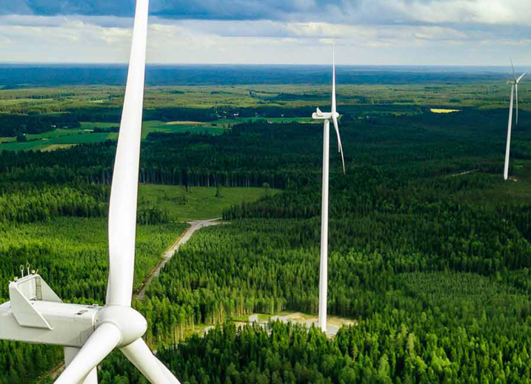
Test grids with varied grid components were implemented to enable variable modelling scenarios. Test grids are run on the simulation platform. With simulations, it is possible to verify and analyse smart grid functions. Different electricity production, consumption and storage profiles can be studied. Wind, solar or, in some cases, both electricity production methods are used in test grids. This is especially useful when observing weather-dependent renewable energy production effects on the grid balance.

How is modelling enabled – components of the simulation platform

The PowerWorld simulator is the brains of our simulation environment. We chose this simulator because we had prior experience with the PowerWorld simulator, which best suited our needs. PowerWorld simulator is an interactive package designed to simulate high-voltage power system operations. It has a graphical user interface (GUI) to build power systems. During the project, we built different power systems in the simulator.

API

In addition to the simulator, we needed an application programming interface (API) to transfer data automatically between the PowerWorld simulator and an Excel spreadsheet. This was solved by the PowerWorld add-on called SimAuto, which serves as the programming interface. With the SimAuto add-on, existing functions were available to facilitate data movement between Excel and PowerWorld. In addition to these existing functions, it was necessary to write other functions. For example, a function that keeps track of a battery’s charge and a progress indicator for the simulation.

Real-life data

We obtained real-life consumption data from an apartment building that we used as a load in our network model. We also got production data from solar and wind power plants. Using real data, we wanted to test whether the fictional PowerWorld model network remains stable when disconnected from the national grid and is balanced using energy storage. In the example case, power generation came from wind and solar energy, and energy storage helped to balance the grid when needed.

Simulation intervals

We placed the collected data into Excel at ten-second intervals and conducted daily or weekly simulations. We transferred the collected data from Excel to PowerWorld for calculation using VBA code. PowerWorld performed the calculations for us and returned results like bus voltage angles and voltages of buses in kilovolts and per units back to Excel. Excel also generated line graphs, displaying how the voltages can change during different simulations and conditions.

User interface

In addition to the programming, a user interface had to be built in Excel to allow users to use the simulation platform. First, the user needs to locate the appropriate PowerWorld binary file (PWB) and open it within the Excel graphical user interface. This action establishes a connection between Excel and PowerWorld, enabling the simulation to start. PowerWorld binary file contains the actual power system data for each case. Each network model has its own Excel files, and there are two different durations for simulations – one-day and one-week-long simulations.

Test grids

We constructed various power system models during the project using the PowerWorld simulator. For example, one of the power system models includes a wind turbine, a solar power plant, a slack generator that balances the power system, and one load which acts as an apartment building area.

Test grid modelling with wind power production

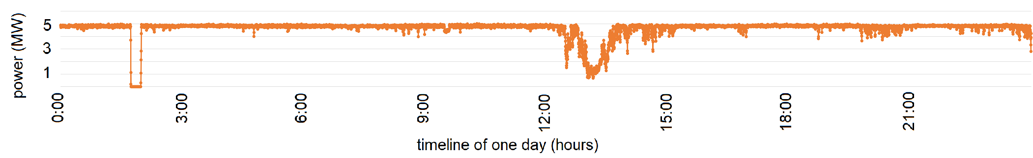
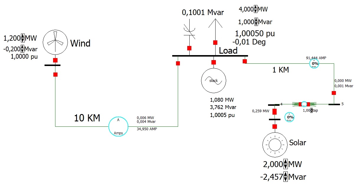
The first test grid is presented in Figure 1. We wanted to start with a simple model, which includes only one production source, one consumption target and one battery energy storage. Production is represented with a 5 MW wind turbine located on the left of the test grid, the profile of which is presented in Figure 2.

Although wind power’s instantaneous values of real and reactive power in Figure 1 are 0,705 MW and 0,180 Mvar, in modelling, the real power followed the profile presented in Figure 2. The load consisted of 70 blocks of flats, and as already mentioned, consumption is based on real-life data.

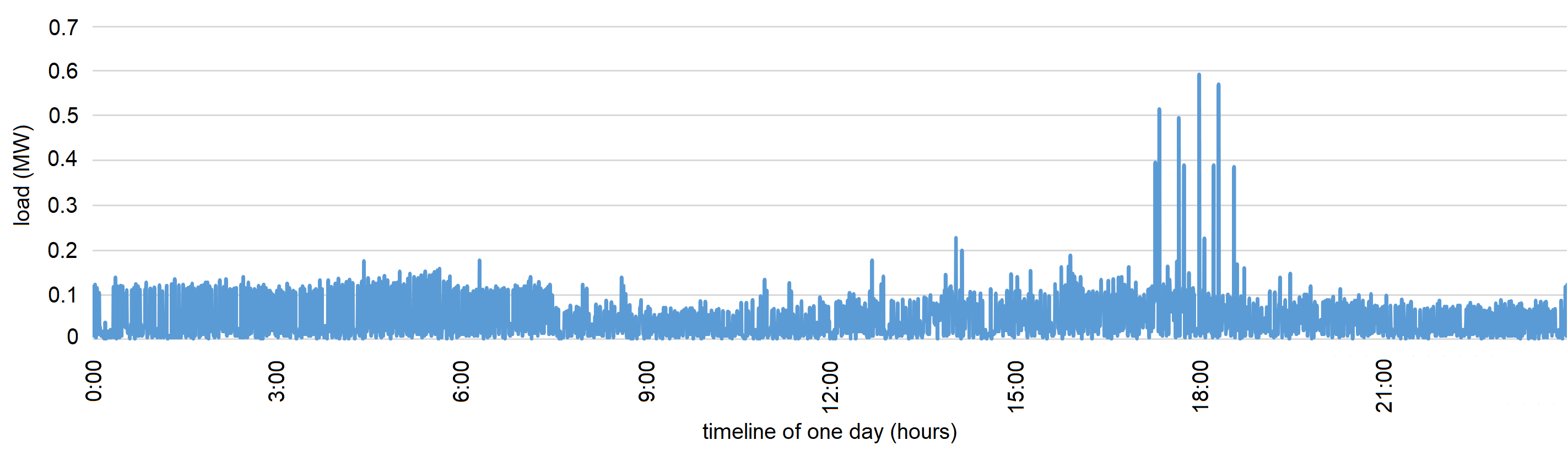
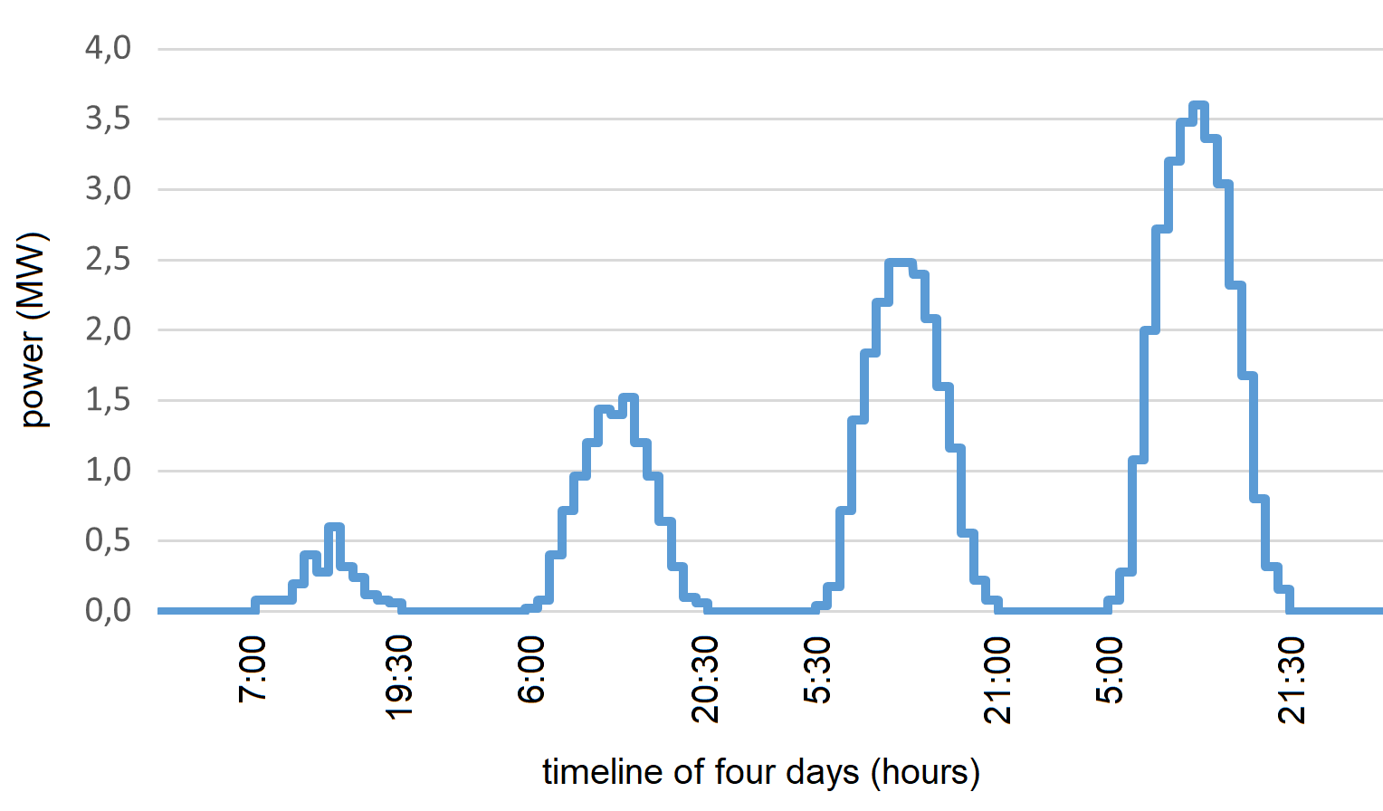
The measured load profile for one building (block of flats) is presented in Figure 3, and as the total load consisted of 70 buildings, in modelling, the profile of Figure 3 was multiplied by 70. The load has a power factor of 0.97 and is located on the right of the test grid. As can be seen, the instantaneous values of real and reactive load power in the figure are 2,0 MW and 0,3 MVar, respectively.

 

 

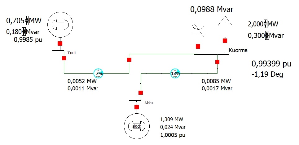
Implementing modelling is such that Powerworld gets the power values of production and consumption as inputs from Excel, after which the steady-state calculations are carried out to compute node voltages of the grid. The power balance has to be fulfilled, which means that the battery energy storage contributes to the required power in the cases of over and underproduction of wind power. A simple prerequisite for the microgrid is that the battery energy storage capacity must remain positive. If the storage becomes empty, it will not be able to maintain the power balance in the grid, which will result in the failure of the electric energy system.

When real and reactive powers of wind production, consumption and battery energy storage are known, the cables will be loaded accordingly, as shown in Figure 1. The modelling time step is 10 s, meaning that energies during each time step are computed by multiplying the powers by 10 s. Then, new inputs from Excel are entered for the powers of production and consumption, and steady-state analysis of the grid is carried out again. By continuing this way, the simulation of one day takes 8640 rounds of calculation, and the corresponding value for one week of simulation is 60480.

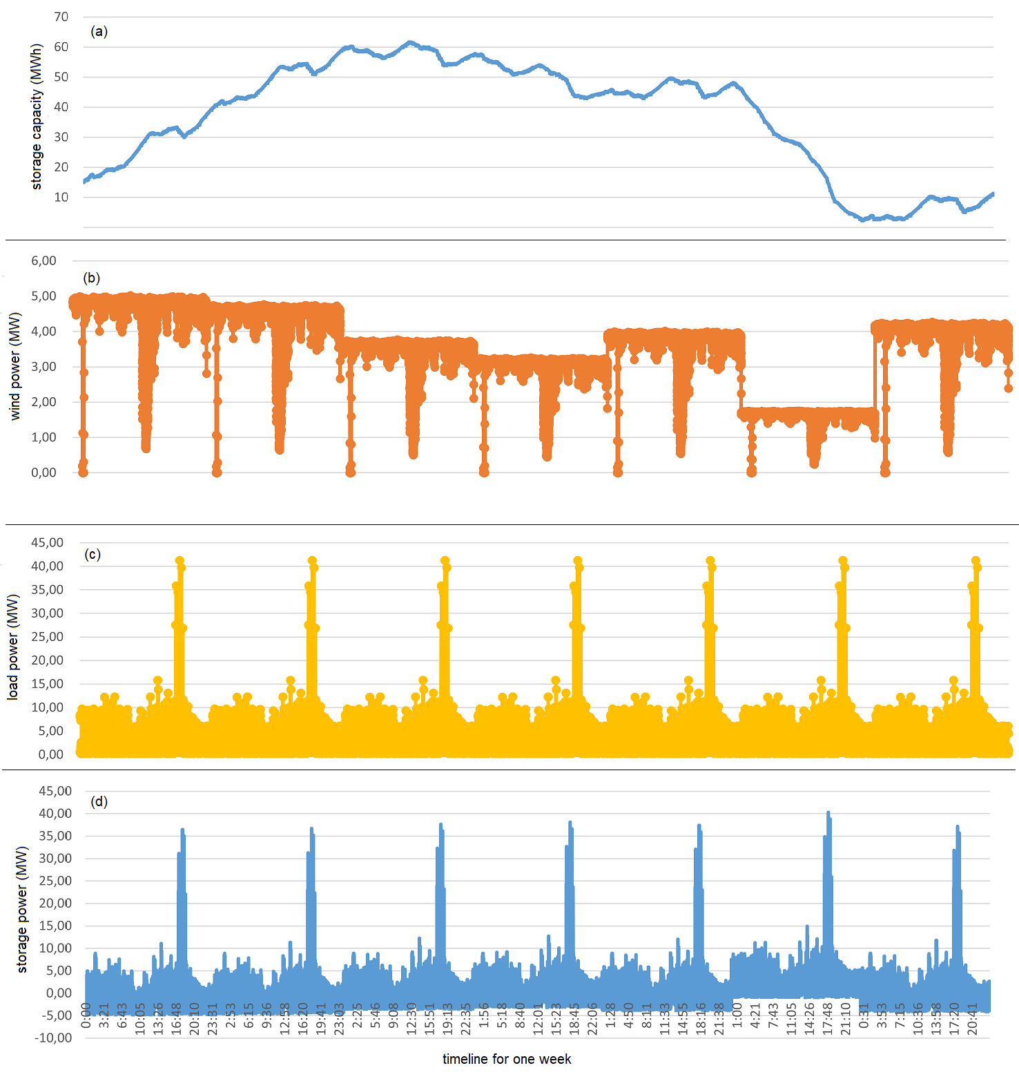
Simulated real power results for a week run are presented in Figure 4. As shown in Figure (b), weather conditions for 5 MW wind power production vary day-by-day with the percentages of 100-95-75-65-80-20-85 corresponding to the data presented in Figure 2.

As the conditions for wind power production are excellent during the first two days, the battery energy storage with the initial capacity of 15 MWh gets charged to about 60 MWh, as seen in Figure (a). Charging takes place during the first two days, since the production power generally exceeds the consumption of 70 blocks of flats. However, occasional discharging also occurs during peak consumption in the evening (Figure (c)).

The power of battery energy storage is presented in Figure (d). When the values are positive, energy is supplied to the grid by discharging the storage, and negative values of power represent the charging of storage. High consumption peaks in the evening are taken from the storage. However, the high amount of data in the figure makes it difficult to see that the storage power values are negative most of the time during the first two days. Consequently, the storage is charged and its capacity increases.

During the third day, the average powers of production and consumption are almost equal since the battery capacity remains relatively steady. Thus, the wind power production of 75% compared to the data presented in Figure 2 results in approximately the same daily average power as the consumption profile of 70 blocks of flats combined with the grid losses. During the fourth day, the conditions for wind power production (65%) continue to degrade, causing the storage capacity to drop below 50 MWh.

fifth day is quite windy (80%) and recovers the storage capacity to about 50 MWh, but the calm wind conditions of the sixth day (20%) result in the heavy discharging of the storage. The failure of the electric energy system during the sixth day is barely avoided, as the storage capacity drops dangerously close to zero. The seventh day saves the situation with wind power production of 80%.

Test grid modelling with wind and solar power production

The second simulation included solar power production in the test grid to support wind power. It is generally known that these two weather-dependent forms of production support each other since windy days are typically not so sunny, and sunny days are typically not so windy (Jervey 2016). As shown from the test grid presented in Figure 5, photovoltaic production with a nominal power of 4 MW is on the right side of the grid. As solar power is produced with a voltage level of 0.4 kV, a 0.4/20 kV transformer is also included. Otherwise, the system and its simulation principles remain the same as in the previous section.

The variation of solar power in different weather conditions is presented in Figure 6. Thus, when considering the solar energy production, we had four different weather conditions for a summer day, and these conditions varied day-by-day in simulations.

The simulated real power results for a one-week run are presented in Figure 7. In this simulation, the weather conditions for 5 MW wind power production varied day-by-day with the percentages of 100-80-60-20-70-40-90 corresponding to the data shown in Figure 2. Consequently, in the four-tier classification of sunniness conditions, the day-by-day variation of solar power with the values of 1-1-3-4-3-4-1 was used.

Grade 1 corresponds to the worst condition with the left-hand profile in Figure 6, whereas Grade 4 corresponds to the best condition with the right-hand profile of Figure 6. With these wind and solar production profiles, calm days are supported by quite high solar power production and cloudy days are supported by relatively high wind power production. The load of the grid was the same as in the previous section. It consisted of 70 blocks of flats, the profile of which was already presented in Figure 4 (c). The mutually supportive characteristics of wind and solar power can be seen in (b) and (c) of Figure 7.

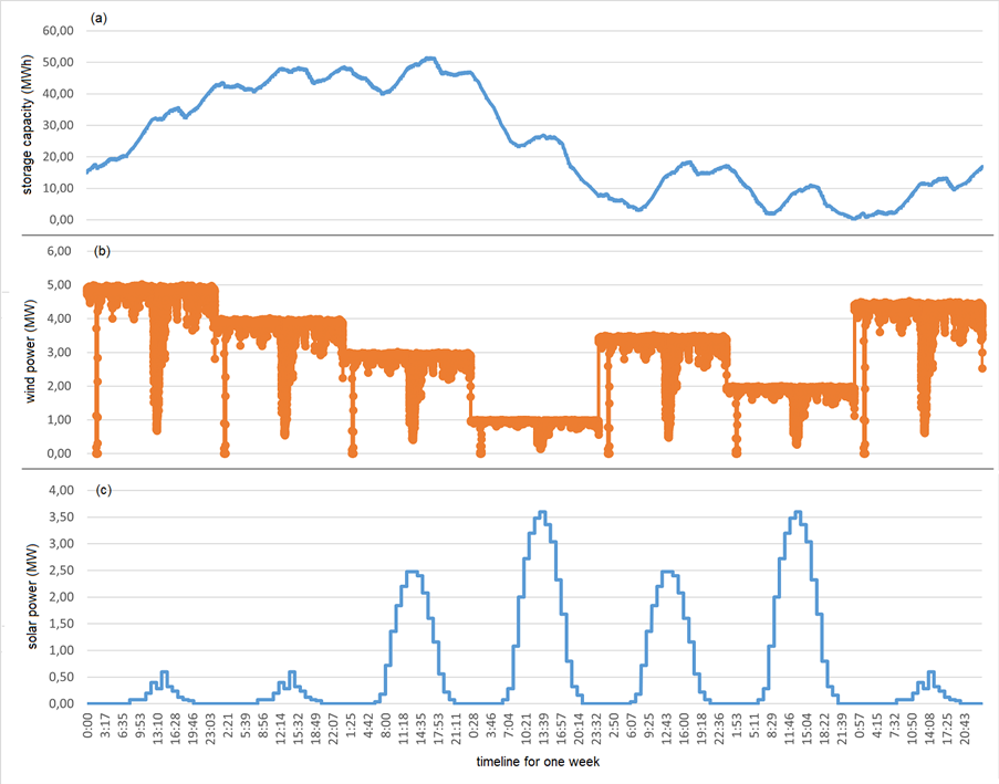
Figure 7 (a) shows that the microgrid stays operational throughout the week since the storage capacity always remains positive. There are no problems during days 1-4, but the breakdown during the fifth day is barely saved by the increased solar power production starting at about 6 am. As can be seen, almost an equivalent occasion is repeated during the sixth day. High peaks of consumption decrease the storage capacity close to zero again in the evening of the sixth day, but the excellent wind conditions barely save the grid breakdown during the seventh day.

How modellings can be utilised?

Simulation platforms and test grids make it possible to model the features of smart grids. Different scenarios and profiles of electricity production, consumption, and storage can be created and studied. Through modelling, it can be discovered how grid balance can be maintained when production and consumption fluctuate according to given values. Thus, the impact of value changes on components can be researched.

Modelling provides valuable information on the properties and limitations of the particular smart grid, especially for renewable energy objects. By modelling, the right component features can be worked out according to needs. Hence, a simulation platform can be used, for example, in grid designing. The properties of the simulation platform are also suitable for educational purposes. Electrical engineering students can utilise the information they gain by executing smart grid modelling. By running test grid simulations, students can observe and analyse the effects of given values on the grid components. Factors affecting the grid balance can be studied. In the project, modelling was piloted in the Smart Grids and Energy Storage -course at Tampere University of Applied Sciences. According to student surveys and interviews, modelling with the simulation platform was useful in teaching, educational development and student learning.

Reference

Jervey, B. 2016. Wind and Solar Are Better Together, Scientific American, December 5 2016, https://www.scientificamerican.com/article/wind-and-solar-are-better-together/